Algorithm | Competitive Paging Algorithm

Notes for Marking algorithms Analysis, Reference: [1] Fiat, A., Karp, R. M., Luby, M., McGeoch, L. A., Sleator, D. D., & Young, N. E. (1991). Competitive paging algorithms.
[2] Achlioptas, D., Chrobak, M., & Noga, J. (2000). Competitive analysis of randomized paging algorithms.

1. Introduction

這篇介紹 Competitive Paging Algorithm，Marking Algorithm 是一種 Online Paging Algorithm，並且是 Randomized Algorithm， 主要目的是用來說明分析這些 Online Paging Algorithm 的工具。詳細的原始論文可以參考 [1] 和 [2]。

所以 Marking Alogrithm 並不是一個實際在 OS 中被廣泛使用的演算法，但透過這對於 Marking Algorithm 的分析，可以更好的了解 Competitive Algorithm 的特性。

• 例如: LRU(Last Recently Used) 就是一種 Marking Algorithm，FIFO(First In First Out) 則不是。

[1] 是首次提出 Competitive Paging Algorithm 與 Marking Algorithm 分析的論文

[2] 則在前三章有對於 Marking Algorithm 的更詳細與緻密的分析

2. Paging Problem

從最開始的 Paging Problem Definition 開始到 Offline Optimal Algorithm, Marking Algorithm 的介紹。

Paging Problem Definition:

1. A two-level memory system, capable of holding $K$ items in the Cache.
2. At each time step, a request to an item is issued.
3. If the item $p$ exists in the Cache, then the cost is 0.
4. If the item $p$ does not exist in the Cache:
   • Choose an item $q$ to replace it, and the cost is 1.

這個問題是一個 Online Problem，因為沒有辦法知道未來的 Request，所以只能根據目前的 Request 來做決策。 但是我們可以先從 Offline Algorithm 開始，來了解這個問題的 Optimal。

2.1 Optimal Algorithm

• 目前被證明的 Belady’s Optimal Algorithm 被證明是 Optimal Algorithm
  • Belady’s Optimal Algorithm 也被稱為 Longest Forward Distance(LFD) Algorithm
• 簡單來說就是把未來最久才會被 Request 的 Item replace

Example:

• Cache Size = 3, Request Seq = { 1,2,3,4,1,2,5,1,2,3,4,5 }

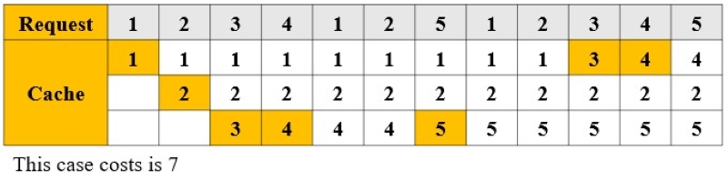
關於 Optimal Algorithm 的證明可以參考 stack overflow:Proof for optimal page replacement (OPT)，使用 Contradiction 來證明 Optimal Algorithm 是最佳的。

但是在現實中我們無法得知一個 item 多久才會被 Request，這個演算法也被稱為 clairvoyant replacement algorithm，因為要做到 Optimal 需要透視未來的 Request。

2.2 Marking Algorithm

這邊我們先給出一個基本的 Marking Algorithm，這是從 [1] 中提出的。

• 假設有一個 Cache，跟大小相同的 Marking Bit Array，用來記錄 p 是否在 Cache 中
• 發生 Request 時，如果 p 已經被 Marked，則 Cost = 0
• 如果 p 沒有被 Marked，則 Cost = 1
  • Total marked item < k，則 Mark p
  • Total marked item = k，則 Unmark all items，然後再 Mark p

Example:

• Cache Size = 3, Request Seq = { 1,2,3,4,1,2,5,1,2,3,4,5 }

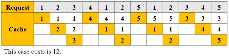
這個 Seq 是故意設計的最糟情況，可以看到 Marking Algorithm 不斷填滿 Array，然後清空。注意我們的重點在於對 Marking Algorithm 的分析，而不是實際的使用。

3. Preliminaries

在分析上會以 [2] 為主要的論文，相較於 [1] 在 1991 剛被提出，到了 [2] 2000 年已經有更多的分析工具。

Throughout this node:

• $k$ denote the size of the cache
• $ALG(𝛼)$ denote the online algorithm

Definition. An online algorithm $ALG$ is $c-competitive$ if, for any instance $I$, $ALG(I) \leq c \cdot OPT(I)$.

• 先定義 $c-competitive$ 的概念，$OPT(I)$ 是最佳的，而 $ALG(I)$ 是 Online Algorithm
  • $\text{If c = 1, ALG is equivalent to OPT}$

3.1 Bounds k-competitive

首先我們先證明任何 Online Algorithm 都是 $k-competitive$，證明其最糟情況下至少是 OPT 的 $k$ 倍。

Theorem. For any $k$ and any deterministic online algorithm $ALG$, the competitive ratio of $ALG \geq k$.

1. A always request the page that is not currently in the cache, This causes a page fault in every access.
2. The total cost of $ALG$ is $|𝛼|$
3. The total cost of $OPT$ is at most $|𝛼|/k$
   • Becase $OPT$ can only a single page fault in any $k$ accesses
4. The base competitive ration is $k$

簡單來說有一個無論如何都會產生 Page fault 的輸入，這樣就可以證明任何 $\text{ALG}$ 最糟情況下都是 $k-competitive$。

3.2 Potential Method

在 Randomized online algorithm 的分析中常常會使用 Amortized Analysis，Paging Problem 也是如此， [2] 中就使用了 Potential Method 來分析 Marking Algorithm 的 Upper Bound。

• Each operation has state $w \text{(work function), } A\text{(ALG conguration), } \text{r(request)}$
• $Δcost_A$ is the cost of $ALG$
• $Δopt$ is the cost of $OPT$
• $Δϕ$ is the potential function change

首先定義每次的操作都會有狀態 $w, A, \text{r}$，然後定義 $Δcost_A, Δopt, Δϕ$ 來分析每次操作的成本。這樣我們就能給出公式:

這個公式就是 Competitive Ratio 的定義，每次操作的成本加上 Potential Function 的變化都應該小於等於 $c$ 倍的 $OPT$。

3.3 Work Function

Work Function 是一個用來描述每次操作的狀態或者是成本的函數，這裡定義 $w(A)$ 來描述 $A$ 的狀態

Lemma. Every offset function is coned up from the set of configurations for which its value is zero. Moreover, if $\omega$ is the current offset function and $r$ is the last request, then there is a sequence of sets $L_1, L_2, \ldots, L_k$, with $L_1 = r$, such that $\omega(X) = 0$ if and only if $|X \cap \bigcup_{i \le j} L_i| \ge j$ for all $1 \le j \le k$.

這裡的 $L$ 代表的是一組 Request 的集合，稱作 Layer，例如: $w(X)=0$ 代表之前的輸入都在 Cache 中，所以 Cost = 0，同樣也有該輸入的 item 數量一定比 $k$ 小。 這裡定義三種集合:

• $V(w) \text{ is mean valid, no cost occurs so the cost is 0}$
• $S(w)=⋃_{i \leq j}L_i \text{ is the set of all requests for this work function}$
• $N(w) \text{ is non-revealed item in } S(w)$

After Request

然後是在 Request 之後的狀態變化，這裡定義 $\omega’$ 來描述 Request 之後的狀態變化。

• $r \in L_j$ 中，則將 $r$ 移到最前面，而 $L_j$ 之後的 Layer 都移除 $r$ 並且加入到 $L_{j+1}$
• $r \in L_k$ 中，則將 $r$ 移到最前面，並且移除 $L_k$
• $r \notin S(\omega)$，則將 $r$ 移到最前面

在之後的分析中，我們會使用這個 Work Function 來描述每次操作的狀態變化，下面會給出一個例子。

這裡也能看處 Request 實際上就 3 種情況

example:

• $\text{Let } k = 3,\text{ {a,b,c} in cache, Request = {d,e,b}}$

• $\text{The optimal cost is 2.}$

4. Analysis

首先我們已經清楚了 Marking Algorithm 的過程，所以有兩個 $Fact$:

Fact 1. The cache contains only marked items and active items. All marked items are in the cache. If there are $m$ marked items and $v$ active items then each active item is in the cache with probability $(k-m)/v$.

Fact 2. Let $w = (L_1|L_2|…|L_k)$ If $L_i$ contains a marked item then all item in $⋃_{j \leq i}L_j$ are marked.

• Fact 1 可以得知 Cache 中的 Active Item 在 Cache 中的機率
• Fact 2 則是說明如果 Layer 中有 Marked Item，則之後的 Layer 都會有 Marked Item

Theorem 2. The competitive ratio of the marking algorithm is $2H_k - 1$.

4.1 Lower Bound

透過最糟情況的設計，來證明 Competitive Ratio 的 Lower Bound。

Proof. A cycle of request $k+1$ items, where the optimal cost 1, while the cost on the Marking Algorithm is $2H_k - 1$.

1. $w = (x_1|x_2|…|x_k)$, Active set $X = {x_1, x_2, …, x_k}$, Marked set $M = {x_1}$
2. $w^y = (y|x_1, x_2| … |x_k)$, Marked set $M = {y, x_1}$
3. Continuous request $x_2, …, x_{k-1}$
   • When ends $w^{k-1}=(x_{k-1}|…|x_2|y|x_1,x_k)$
   • Marked set $M = {x_{k-1},…,x_2,x_1,y}$, size $k-1$
4. Last Request $x_k$
   • Marked set is full, so unmark all items.
   • The cost must be 1.

先設計一個 k+1 個 Request，首先 cache 中已經存在 $x_1$。首先 Request $y$ 然後再 Request $x_2, …, x_k$， 因為是從 $k_2, …, x_k$ 不斷去請求，因此分母會不斷減少，最後一次 Request $x_k$ 則必然會產生 Cost = 1。以此得到以上的公式，是一個 Harmonic Number， 所以可以得到 $\text{Competitive Ratio} = 2H_k - 1 \approx 2ln(k) - 1$。

4.2 Upper Bound

在 [2] 中更使用 Potential Method 來證明 Competitive Ratio 的 Upper Bound，證明了 $2H_k - 1$ 是 Tight

Proof. Prove that Marking Algorithm is $2H_k - 1$ competitive, using Potential Method.

如果當前的 Work Function 有 $s$ 個 Layer，且包含未標記的 Item，則 Potential Function 為:

• Potential Function $ϕ(w) = s(H_k - H_s + 1)$
  • $H_k, H_s$ is Harmonic Number of $k, s$
  • $s$ is the number of layers for work function $w$

首先把 Request 分成 3 種情況:

• (a) Request outside the $S(w)$, $t$ is the number of (a)
• (b) Request in the $S(w)$ but not in the cache, $l$ is the number of (b)
• (c) Request in the cache

最後是我們證明的目標:

完成以上的定義後我們就能來分析 Request 的情況。

Class (a)

$r \notin S(w)$, 這裡給個例子來說明什麼是 Class (a) 的 Request:

• Example $k = 3, M = \text{{a, b, c}}, \text{Request} = \text{{d}}$
  • $(a|b|c) \rightarrow (d|a,b|c)$

這裡可以看出 (a) 其實就是一定會產生 Cost 的 Request，並且從此我們能看出 $Δopt = t$，實際上 $t$ 就是 OPT 的 Cost。

Class (b)

$r \in S(w), r \notin M(w)$, 同樣用例子來說明 Class (b) 的 Request:

• Example $k = 3, M = \text{{a, b}}, Request = \text{{c}}$
  • $(a|b|c) \rightarrow (c|a,b|)$

這裡根據 Fact 2. Class (b) 可以使 $s$ 減少 1，所以將會有 $l \leq s$。

Class (c)

$r \in S(w), r \in M(w)$, C 是已經被 Marked 的 Item，所以實際上不會有變化。

• 如果出現一個 $\text{Class (c) i}$ Request，則最多會有 $l+t+i-1$ 個 Marked Item
  • 因為 (a), (b) 最多貢獻 $l+t$ 個 Marked Item，而 $i$ 則是 Class (c) 的 Request
• 同時 Active item 的數量會是 $k-i+1$
• 根據 Fact 1. 得出這次請求的 Cost = 1 的機率是 $(l+t+i-1)/(k-i+1) = (l+i)/(k-i+1)$

因為 i 的範圍是從 1 到 $k-l-t$，所以可以得到以下公式:

上面用 Harmonic Number 來表示，這裡的 $H_k - H_{l+t}$ 是因為 $\sum_{i=1}^{k} \frac{1}{i} = H_k$，所以這裡是 $H_k - H_{l+t}$

Upper bound

這樣我們就算出了所有的 Request 的 Cost，然後再加上 Potential Function 的變化，就能得到 $(2H_{k-1}) \cdot Δopt$ 的部分， 跟以下的不等式:

• (1) 是來自於 $\Delta cost$ 的界線以及 $\Phi ,s,s’$ 的定義
• (2) $l \leq s$ 並且 $\Phi$ 隨著 $s$ 增加而增加
• (3) 因為 $2t - (l+t)H_{l+t} \leq -lH_{l+1}$ 跟 $s’ \leq t$

以上就是透過分析 Marking Algorithm 的 Upper/Lower Bound，Competitive Ratio = $2H_k - 1$ 並且是 Tight 的證明。

這個 Marking Algorithm 只是一個最簡單的例子來說明 Competitive Paging Algorithm 的分析，實際上在 OS 中 Marking Algorithm 還有更多的變化， 通常更多的透過 Learning strategy 來做決策，例如: Clock-PRO，在分析上大部分是基於實驗的方式。

Last Edit

06-21-2024 09:07